LoRA简介
 
通过调整小规模低秩子集的模型参数，优化预训练模型以适应特定数据集

减少大型模型在任务特定数据上的微调计算成本和时间
 
LoRA工作原理
 
在训练过程中，通过学习一个近似的权重更新矩阵(ΔW)来高效计算权重更新 
LoRA通过学习两个小的权重矩阵(A)和(B)来实现这一目标，从而节省GPU内存
 
DoRA简介
 
DoRA是LoRA的一种改进，基于方向向量(V)和幅度向量(m)的分解进行微调
 
 
目的是提高模型对方向变化的适应能力，同时保持参数效率
 
实现LoRA层
 
使用PyTorch模块实现LoRA层，便于替换现有神经网络中的线性层
LoRALayer类用于初始化A和B矩阵，以及α缩放超参数和秩超参数
 
实现DoRA层
 
将LinearWithLoRAMerged类升级为LinearWithDoRAMerged
引入动态归一化和缩放步骤以改善训练性能
 
 
添加可学习的幅度向量self.m
 
应用实例
 
在多层感知器中应用LoRA和DoRA层，通过冻结原始线性层并仅使LoRA层可训练来优化模型训练过程
 
结论与展望
 
DoRA被视为LoRA的有效扩展，具有更高的参数效率和更好的鲁棒性
 
 
对于未来在LLM微调中的实际应用充满期待

原文https://sebastianraschka.com/blog/2024/lora-dora.html

Low-rank adaptation (LoRA) is a machine learning technique that modifies a pretrained model (for example, an LLM or vision transformer) to better suit a specific, often smaller, dataset by adjusting only a small, low-rank subset of the model’s parameters.
低秩适应 (LoRA) 是一种机器学习技术，它通过仅调整一个小的、低的数据集来修改预训练模型（例如 LLM 或视觉变换器），以更好地适应特定的、通常较小的数据集。 -模型参数的排名子集。

This approach is important because it allows for efficient finetuning of large models on task-specific data, significantly reducing the computational cost and time required for finetuning.
这种方法很重要，因为它允许对特定于任务的数据对大型模型进行有效的微调，从而显着减少微调所需的计算成本和时间。

Last week, researchers proposed DoRA: Weight-Decomposed Low-Rank Adaptation, a new alternative to LoRA, which may outperform LoRA by a large margin.
上周，研究人员提出了 DoRA：权重分解低阶自适应，这是 LoRA 的新替代方案，其性能可能会大幅优于 LoRA。

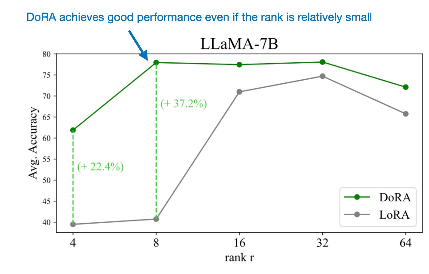
DoRA is a promising alternative to standard LoRA (annotated figure from the DoRA paper: https://arxiv.org/abs/2402.09353)
DoRA 是标准 LoRA 的一个有前途的替代方案（来自 DoRA 论文的注释图：https://arxiv.org/abs/2402.09353）

To understand how these methods work, we will implement both LoRA and DoRA in PyTorch from scratch in this article!
为了了解这些方法的工作原理，我们将在本文中从头开始在 PyTorch 中实现 LoRA 和 DoRA！

LoRA Recap   洛拉回顾

Before we dive into DoRA, here’s a brief recap of how LoRA works.
在我们深入了解 DoRA 之前，先简要回顾一下 LoRA 的工作原理。

Since LLMs are large, updating all model weights during training can be expensive due to GPU memory limitations. Suppose we have a large weight matrix WW for a given layer. During backpropagation, we learn a ΔWΔW matrix, which contains information on how much we want to update the original weights to minimize the loss function during training.
由于 LLMs 很大，因此由于 GPU 内存限制，在训练期间更新所有模型权重的成本可能会很高。假设给定层我们有一个很大的权重矩阵 WW 。在反向传播期间，我们学习一个 ΔWΔW 矩阵，其中包含有关我们想要在训练期间最小化损失函数的原始权重的更新程度的信息。

In regular training and finetuning, the weight update is defined as follows:
在常规训练和微调中，权重更新定义如下：

The LoRA method proposed by Hu et al. offers a more efficient alternative to computing the weight updates ΔWΔW by learning an approximation of it, ΔW≈ABΔW≈AB. In other words, in LoRA, we have the following, where AA and BB are two small weight matrices:
Hu等人提出的LoRA方法。通过学习权重更新的近似值 ΔW≈ABΔW≈AB ，提供了一种更有效的替代方法来计算权重更新 ΔWΔW 。换句话说，在 LoRA 中，我们有以下内容，其中 AA 和 BB 是两个小权重矩阵：

(The “.” in “A.BA.B” stands for matrix multiplication.)
（“ A.BA.B ”中的“.”代表矩阵乘法。）

The figure below illustrates these formulas for full finetuning and LoRA side by side.
下图并排说明了完全微调和 LoRA 的这些公式。

An illustration of regular finetuning (left) and LoRA finetuning (right)
常规微调（左）和 LoRA 微调（右）示意图

How does LoRA save GPU memory? If a pretrained weight matrix WW is a 1,000×1,000 matrix, then the weight update matrix ΔWΔW in regular finetuning is a 1,000×1,000 matrix as well. In this case, ΔWΔW has 1,000,000 parameters. If we consider a LoRA rank of 2, then AA is a 1000×2 matrix, and BB is a 2×1000 matrix, and we only have 2×2×1,000 = 4,000 parameters that we need to update when using LoRA. In the previous example, with a rank of 2, that’s 250 times fewer parameters.
LoRA如何节省GPU内存？如果预训练的权重矩阵 WW 是一个1,000×1,000的矩阵，那么常规微调中的权重更新矩阵 ΔWΔW 也是一个1,000×1,000的矩阵。在本例中， ΔWΔW 有 1,000,000 个参数。如果我们考虑 LoRA 秩为 2，则 AA 是一个 1000×2 矩阵， BB 是一个 2×1000 矩阵，我们只有 2×2×1,000 = 4,000使用LoRA时我们需要更新的参数。在前面的示例中，等级为 2，参数数量减少了 250 倍。

Of course, AA and BB can’t capture all the information that ΔWΔW could capture, but this is by design. When using LoRA, we hypothesize that the model requires W to be a large matrix with full rank to capture all the knowledge in the pretraining dataset. However, when we finetune an LLM, we don’t need to update all the weights and capture the core information for the adaptation in a smaller number of weights than ΔWΔW would; hence, we have the low-rank updates via ABAB.
当然， AA 和 BB 无法捕获 ΔWΔW 可以捕获的所有信息，但这是设计使然。当使用 LoRA 时，我们假设模型需要 W 是一个满秩的大矩阵，以捕获预训练数据集中的所有知识。然而，当我们微调LLM时，我们不需要更新所有权重并以比 ΔWΔW 更少的权重捕获适应的核心信息；因此，我们通过 ABAB 获得低排名更新。

If you paid close attention, the full finetuning and LoRA depictions in the figure above look slightly different from the formulas I have shown earlier. That’s due to the distributive law of matrix multiplication: we don’t have to add the weights with the updated weights but can keep them separate. For instance, if xx is the input data, then we can write the following for regular finetuning:
如果您仔细观察，上图中的完整微调和 LoRA 描述看起来与我之前展示的公式略有不同。这是由于矩阵乘法的分配律：我们不必将权重与更新的权重相加，而是可以将它们分开。例如，如果 xx 是输入数据，那么我们可以编写以下代码进行常规微调：

Similarly, we can write the following for LoRA:
同样，我们可以为 LoRA 编写以下内容：

The fact that we can keep the LoRA weight matrices separate makes LoRA especially attractive. In practice, this means that we don’t have to modify the weights of the pretrained model at all, as we can apply the LoRA matrices on the fly. This is especially useful if you are considering hosting a model for multiple customers. Instead of having to save the large updated models for each customer, you only have to save a small set of LoRA weights alongside the original pretrained model.
事实上，我们可以将 LoRA 权重矩阵分开，这使得 LoRA 特别有吸引力。实际上，这意味着我们根本不必修改预训练模型的权重，因为我们可以即时应用 LoRA 矩阵。如果您正在考虑为多个客户托管模型，这尤其有用。您不必为每个客户保存大型更新模型，只需在原始预训练模型旁边保存一小部分 LoRA 权重即可。

To make this less abstract and to provide additional intuition, we will implement LoRA in code from scratch in the next section.
为了减少抽象并提供额外的直观性，我们将在下一节中从头开始在代码中实现 LoRA。

A LoRA Layer Code Implementation
LoRA 层代码实现

We begin by initializing a LoRALayer that creates the matrices A and B, along with the alpha scaling hyperparameter and the rank hyperparameters. This layer can accept an input and compute the corresponding output, as illustrated in the figure below.
我们首先初始化一个 LoRALayer ，它创建矩阵 A 和 B，以及 alpha 缩放超参数和排名超参数。该层可以接受输入并计算相应的输出，如下图所示。

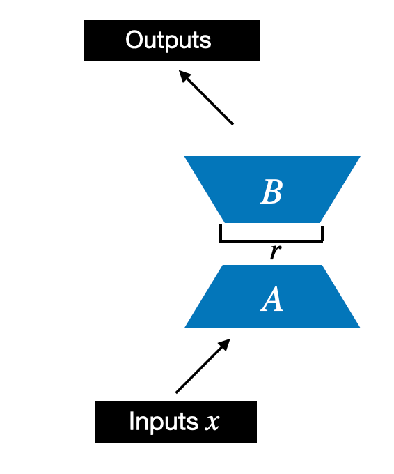
Illustration of the LoRA matrices A and B with rank r
秩为 r 的 LoRA 矩阵 A 和 B 的图示

In code, this LoRA layer depicted in the figure above looks like as follows:
在代码中，上图所示的 LoRA 层如下所示：

In the code above, rank is a hyperparameter that controls the inner dimension of the matrices A and B. In other words, this parameter controls the number of additional parameters introduced by LoRA and is a key factor in determining the balance between model adaptability and parameter efficiency.
上面的代码中， rank 是一个超参数，控制矩阵A和B的内部维度。换句话说，这个参数控制着LoRA引入的额外参数的数量，是决定模型适应性和参数效率之间的平衡。

The second hyperparameter, alpha, is a scaling hyperparameter applied to the output of the low-rank adaptation. It essentially controls the extent to which the adapted layer’s output is allowed to influence the original output of the layer being adapted. This can be seen as a way to regulate the impact of the low-rank adaptation on the layer’s output.
第二个超参数 alpha 是应用于低秩自适应输出的缩放超参数。它本质上控制了适应层的输出允许影响正在适应的层的原始输出的程度。这可以被视为调节低秩适应对层输出的影响的一种方法。

So far, the LoRALayer class we implemented above allows us to transform the layer inputs x. However, in LoRA, we are usually interested in replacing existing Linear layers so that the weight update is applied to the existing pretrained weights, as shown in the figure below:
到目前为止，我们上面实现的 LoRALayer 类允许我们转换层输入 x 。然而，在LoRA中，我们通常感兴趣的是替换现有的 Linear 层，以便将权重更新应用于现有的预训练权重，如下图所示：

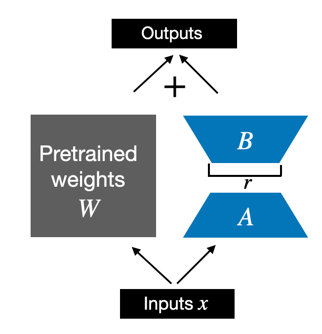
LoRA applied to an existing linear layer
LoRA 应用于现有的线性层

To incorporate the original Linear layer weights as shown in the figure above, we will implement a LinearWithLoRA layer that uses the previously implemented LoRALayer and can be used to replace existing Linear layers in a neural network, for example, the self-attention module or feed forward modules in an LLM:
为了合并上图所示的原始 Linear 层权重，我们将实现一个 LinearWithLoRA 层，该层使用之前实现的 LoRALayer 并可用于替换现有的 Linea 中的自注意力模块或前馈模块：

Note that since we initialize the weight matrix B (self.B in LoraLayer) with zero values in the LoRA layer, the matrix multiplication between A and B results in a matrix consisting of 0’s and doesn’t affect the original weights (since adding 0 to the original weights does not modify them).
请注意，由于我们在 LoRA 层中使用零值初始化权重矩阵 B（ LoraLayer 中的 self.B ），因此 A 和 B 之间的矩阵乘法会生成一个由 0 组成的矩阵，并且不会不影响原始权重（因为向原始权重添加 0 不会修改它们）。

Let’s try out LoRA on a small neural network layer represented by a single Linearlayer:
让我们在由单个 Linear 层表示的小型神经网络层上尝试 LoRA：

In:

Out: 出去：

Now, applying LoRA to the Linear layer, we see that the results are the same since we haven’t trained the LoRA weights yet. In other words, everything works as expected:
现在，将 LoRA 应用于 Linea r 层，我们看到结果是相同的，因为我们还没有训练 LoRA 权重。换句话说，一切都按预期进行：

In:

Out: 出去：

Earlier, I mentioned the distributive law of matrix multiplication:
前面我提到了矩阵乘法的分配律：

x.(W+A.B)=x.W+x.A.Bx.(W+A.B)=x.W+x.A.B.

Here, this means that we can also combine or merge the LoRA matrices and original weights, which should result in an equivalent implementation. In code, this alternative implementation to the LinearWithLoRA layer looks as follows:
在这里，这意味着我们还可以组合或合并 LoRA 矩阵和原始权重，这应该会产生等效的实现。在代码中， LinearWithLoRA 层的替代实现如下所示：

In short, LinearWithLoRAMerged computes the left side of the equation x.(W+A.B)=x.W+x.A.Bx.(W+A.B)=x.W+x.A.B whereas LinearWithLoRA computes the right side – both are equivalent.
简而言之， LinearWithLoRAMerged 计算等式 x.(W+A.B)=x.W+x.A.Bx.(W+A.B)=x.W+x.A.B 的左侧，而 LinearWithLoRA 计算右侧 - 两者是等效的。

We can verify that this results in the same outputs as before via the following code:
我们可以通过以下代码验证这会产生与之前相同的输出：

In:

Out: 出去：

Now that we have a working LoRA implementation let’s see how we can apply it to a neural network in the next section.
现在我们已经有了一个可行的 LoRA 实现，让我们在下一节中看看如何将其应用到神经网络中。

Applying LoRA Layers
应用 LoRA 层

Why did we implement LoRA in the manner described above using PyTorch modules? This approach enables us to easily replace a Linear layer in an existing neural network (for example, the feed forward or attention modules of a Large Language Model) with our new LinearWithLoRA (or LinearWithLoRAMerged) layers.
为什么我们要使用 PyTorch 模块以上述方式实现 LoRA？这种方法使我们能够轻松地用新的 LinearWithLoRA （或 < b2> ) 层。

For simplicity, let’s focus on a small 3-layer multilayer perceptron instead of an LLM for now, which is illustrated in the figure below:
为了简单起见，我们暂时关注一个小型 3 层多层感知器，而不是 LLM，如下图所示：

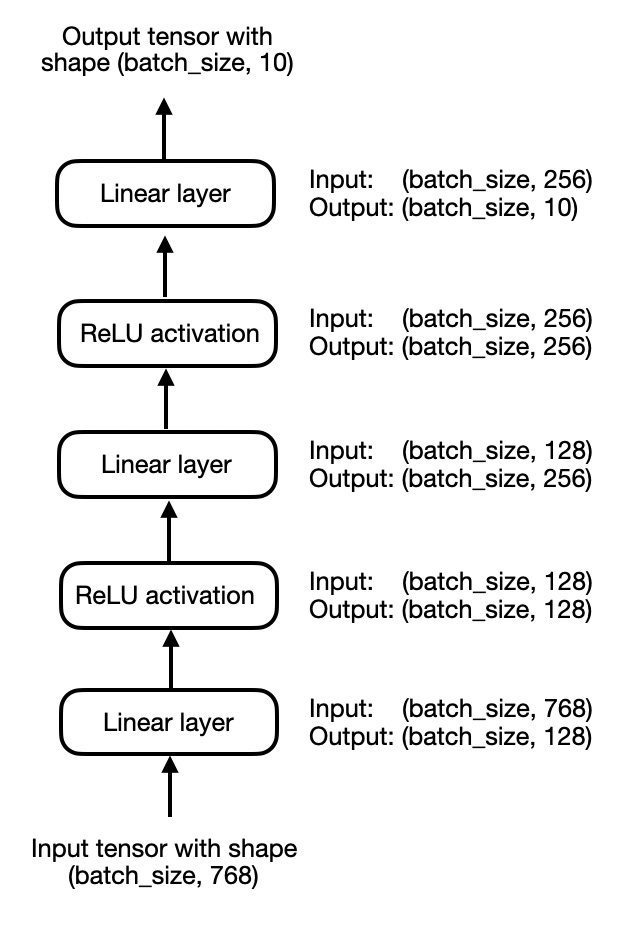
A simple 3-layer multilayer perceptron
一个简单的 3 层多层感知器

In code, we can implement the multilayer perceptron, shown above, as follows:
在代码中，我们可以实现如上所示的多层感知器，如下所示：

In:

Out: 出去：

Using LinearWithLora, we can then add the LoRA layers by replacing the original Linear layers in the multilayer perceptron model:
使用 LinearWithLora ，我们可以通过替换多层感知器模型中的原始 Linear 层来添加 LoRA 层：

In:

Out: 出去：

Then, we can freeze the original Linear layers and only make the LoRALayer layers trainable, as follows:
然后，我们可以冻结原始的 Linear 层，只使 LoRALaye r 层可训练，如下所示：

In:

Out: 出去：

Based on the True and False values above, we can visually confirm that only the LoRA layers are trainable now (True means trainable, False means frozen). In practice, we would then train the network with this LoRA configuration on a new dataset or task.
根据上面的 True 和 False 值，我们可以直观地确认现在只有 LoRA 层是可训练的（ True 表示可训练， False 表示冻结）。在实践中，我们将在新的数据集或任务上使用此 LoRA 配置来训练网络。

To avoid making this a very long article, I am skipping over the boilerplate code to train this model. But if you are interested in the full code, you can find a standalone code notebook here: https://github.com/rasbt/dora-from-scratch.
为了避免这篇文章变得很长，我跳过了样板代码来训练这个模型。但如果您对完整代码感兴趣，可以在这里找到独立的代码笔记本：https://github.com/rasbt/dora-from-scratch。

Furthermore, if you are interested in a LoRA from scratch explanation and application to an LLM, also check out my Lightning Studio LoRA From Scratch – Implement Low-Rank Adaptation for LLMs in PyTorch.
此外，如果您对 LoRA 从头开始​​的解释和 LLM 的应用感兴趣，还可以查看我的 Lightning Studio LoRA From Scratch – Implement Low-Rank Adaptation for LLMs in PyTorch。

Understanding Weight-Decomposed Low-Rank Adaptation (DoRA)
了解权重分解低秩适应 (DoRA)

You may have noticed that we spent a lot of time implementing and talking about LoRA. That’s because DoRA (Weight-Decomposed Low-Rank Adaptation) can be seen as an improvement or extension of LoRA that is built on top of it, and we can now easily adapt some of our previous code to implement DoRA.
您可能已经注意到，我们花了很多时间来实现和讨论 LoRA。这是因为 DoRA（权重分解低秩适应）可以被视为构建在其之上的 LoRA 的改进或扩展，我们现在可以轻松地调整之前的一些代码来实现 DoRA。

DoRA can be described in two steps, where the first step is to decompose a pretrained weight matrix into a magnitude vector (mm) and a directional matrix (VV). The second step is applying LoRA to the directional matrix VV and training the magnitude vector mm separately.
DoRA 可以分两步描述，第一步是将预训练的权重矩阵分解为幅度向量 ( mm ) 和方向矩阵 ( VV )。第二步是将LoRA应用于方向矩阵 VV 并单独训练幅度向量 mm 。

The decomposition into magnitude and directional components is inspired by the mathematical principle that any vector can be represented as the product of its magnitude (a scalar value indicating its length) and its direction (a unit vector indicating its orientation in space).
幅度和方向分量的分解受到数学原理的启发，即任何向量都可以表示为其幅度（指示其长度的标量值）和其方向（指示其空间方向的单位向量）的乘积。

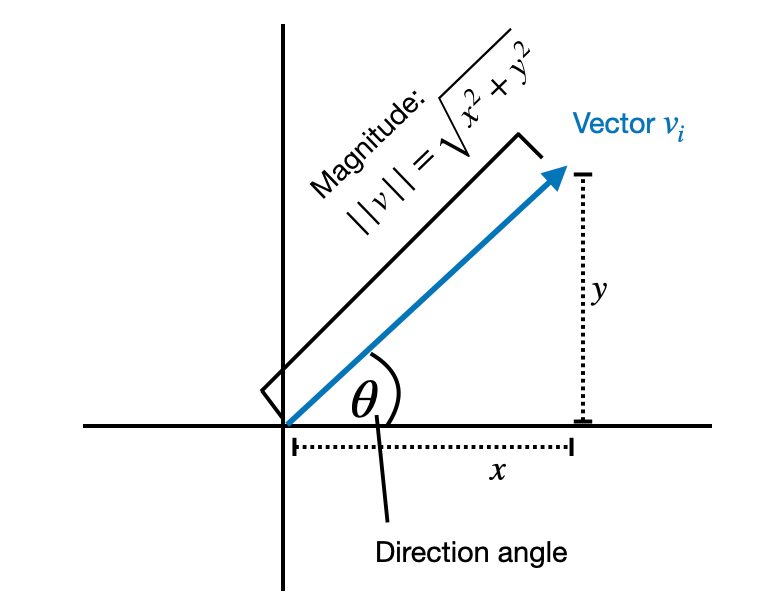
Illustration of the direction and magnitude of a single vector.
单个向量的方向和大小的图示。

For example, if have a 2D vector [1, 2], we can decompose it into a magnitude 2.24 and a directional vector [0.447,0.894][0.447,0.894]. Then 2.24×[0.447,0.894]=[1,2]2.24×[0.447,0.894]=[1,2].
例如，如果有一个 2D 向量 [1, 2]，我们可以将其分解为幅度 2.24 和方向向量 [0.447,0.894][0.447,0.894] 。然后 2.24×[0.447,0.894]=[1,2]2.24×[0.447,0.894]=[1,2] 。

In DoRA, we apply the decomposition into magnitude and directional components to a whole pretrained weight matrix WW instead of a vector, where each column (vector) of the weight matrix corresponds to the weights connecting all inputs to a particular output neuron.
在 DoRA 中，我们将分解为幅度和方向分量应用于整个预训练的权重矩阵 WW 而不是向量，其中权重矩阵的每一列（向量）对应于将所有输入连接到特定的权重输出神经元。

So, the result of decomposing WW is a magnitude vector mm that represents the scale or length of each column vector in the weight matrix, as illustrated in the figure below.
因此，分解 WW 的结果是一个幅值向量 mm ，它表示权重矩阵中每个列向量的尺度或长度，如下图所示。

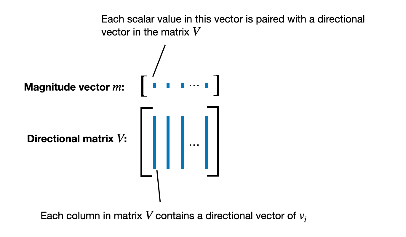
Illustration of the weight matrix decomposition in DoRA
DoRA中权重矩阵分解图解

Then, DoRA takes the directional matrix VV and applies standard LoRA, for instance:
然后，DoRA 采用方向矩阵 VV 并应用标准 LoRA，例如：

The normalization, which I abbreviated as “norm” to not further complicate things in this overview, is based on the weight normalization method proposed in Saliman’s and Kingma’s 2016 Weight Normalization: A Simple Reparameterization to Accelerate Training of Deep Neural Networks paper.
归一化（我在本概述中将其缩写为“范数”，以免使事情进一步复杂化）基于 Saliman 和 Kingma 2016 年的《权重归一化：加速深度神经网络训练的简单重新参数化》论文中提出的权重归一化方法。

The DoRA two-step process (decomposing a pretrained weight matrix and applying LoRA to the directional matrix) is further illustrated in the figure from the DoRA paper below.
下面 DoRA 论文的图中进一步说明了 DoRA 的两步过程（分解预训练的权重矩阵并将 LoRA 应用于方向矩阵）。

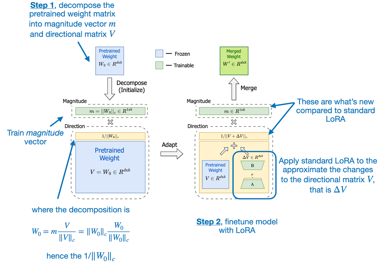
Annotated illustration from the DoRA paper (https://arxiv.org/abs/2402.09353)
DoRA 论文中的注释插图 (https://arxiv.org/abs/2402.09353)

The motivation for developing DoRA is based on analyzing and comparing the LoRA and full finetuning learning patterns. The DoRA authors found that LoRA either increases or decreases magnitude and direction updates proportionally but seems to lack the capability to make only subtle directional changes as found in full finetuning. Hence, the researchers propose the decoupling of magnitude and directional components.
开发 DoRA 的动机是基于对 LoRA 和完全微调学习模式的分析和比较。 DoRA 作者发现，LoRA 会按比例增加或减少幅度和方向更新，但似乎缺乏在完全微调中仅进行细微方向变化的能力。因此，研究人员提出将幅度和方向分量解耦。

In other words, their DoRA method aims to apply LoRA only to the directional component, VV, while also allowing the magnitude component, mm, to be trained separately.
换句话说，他们的 DoRA 方法旨在仅将 LoRA 应用于方向分量